(ENG) The basics of Spark PART 1

Written by Tuyen on 27 Jun 2021

Đầu tiên phải kết nối với Cluster. Cluster được host trên remote machine mà được connect với tất cả các node khác. Sẽ có 1 máy tính gọi là master phụ trách việc bóc tách dữ liệu và tính toán. master được kết nối với tất cả những máy tính còn lại trong cluster, các máy tính còn lại gọi là worker. master gửi cho workers data và các phép toán để chạy và chúng sẽ trả về cho master kết quả.
The first step in using Spark is connecting to a cluster.

In practice, the cluster will be hosted on a remote machine that’s connected to all other nodes. There will be one computer, called the master that manages splitting up the data and the computations. The master is connected to the rest of the computers in the cluster, which are called worker. The master sends the workers data and calculations to run, and they send their results back to the master.

Deciding whether or not Spark is the best solution for your problem takes some experience, but you can consider questions like:

Is my data too big to work with on a single machine?
Can my calculations be easily parallelized?

Bước 1: Create an instance of the SparkContext class to connect to a Spark cluster from PySpark.The class constructor takes a few optional arguments that allow you to specify the attributes of the cluster you’re connecting to.

An object holding all these attributes can be created with the SparkConf() constructor. Take a look at the documentation for all the details! You can think of the SparkContext as your connection to the cluster and the SparkSession as your interface with that connection.

from pyspark.sql import SparkSession, SQLContext

# Create SparkSession. Creating multiple SparkSessions and SparkContexts can cause issues, so it's best practice to use the SparkSession.builder.getOrCreate() method. This returns an existing SparkSession if there's already one in the environment, or creates a new one if necessary!
spark = SparkSession.builder.appName("CAR DAILY").getOrCreate()

# Create sparkContext
sc = spark.sparkContext

sqlContext = SQLContext(sc)

# Verify SparkContext
print(sc)

# Print Spark version
print(sc.version)

<SparkContext master=local[*] appName=pyspark-shell>

You may also find that running simpler computations might take longer than expected. That’s because all the optimizations that Spark has under its hood are designed for complicated operations with big data sets. That means that for simple or small problems Spark may actually perform worse than some other solutions!

Using DataFrames

Spark’s core data structure is the Resilient Distributed Dataset (RDD). This is a low level object that lets Spark work its magic by splitting data across multiple nodes in the cluster. However, RDDs are hard to work with directly, so in this course you’ll be using the Spark DataFrame abstraction built on top of RDDs.

The Spark DataFrame was designed to behave a lot like a SQL table (a table with variables in the columns and observations in the rows). Not only are they easier to understand, DataFrames are also more optimized for complicated operations than RDDs.

When you start modifying and combining columns and rows of data, there are many ways to arrive at the same result, but some often take much longer than others. When using RDDs, it’s up to the data scientist to figure out the right way to optimize the query, but the DataFrame implementation has much of this optimization built in!

To start working with Spark DataFrames, you first have to create a SparkSession object from your SparkContext. You can think of the SparkContext as your connection to the cluster and the SparkSession as your interface with that connection.

I. SELECT

flights.select(flights.air_time/60)

returns a column of flight durations in hours instead of minutes.

if you wanted to .select() the column duration_hrs (which isn’t in your DataFrame) you could do

flights.select((flights.air_time/60).alias(“duration_hrs”))

The equivalent Spark DataFrame method .selectExpr() takes SQL expressions as a string:

flights.selectExpr(“air_time/60 as duration_hrs”) with the SQL as keyword being equivalent to the .alias() method. To select multiple columns, you can pass multiple strings.

View tables: Once you’ve created a SparkSession, you can start poking around to see what data is in your cluster!

Your SparkSession has an attribute called catalog which lists all the data inside the cluster. This attribute has a few methods for extracting different pieces of information.

One of the most useful is the .listTables() method, which returns the names of all the tables in your cluster as a list.

spark.catalog.listTables()

Querying: Running a query on this table is as easy as using the .sql() method on your SparkSession. This method takes a string containing the query and returns a DataFrame with the results!

If you look closely, you’ll notice that the table flights dataframe is only mentioned in the query, not as an argument to any of the methods. This is because there isn’t a local object in your environment that holds that data, so it wouldn’t make sense to pass the table as an argument.

Convert Spark DF to Pandas DF - Pandafy a Spark DataFrame

Suppose you’ve run a query on your huge dataset and aggregated it down to something a little more manageable.

Sometimes it makes sense to then take that table and work with it locally using a tool like pandas. Spark DataFrames make that easy with the .toPandas() method. Calling this method on a Spark DataFrame returns the corresponding pandas DataFrame. It’s as simple as that!

This time the query counts the number of flights to each airport from SEA and PDX.

Remember, there’s already a SparkSession called spark in your workspace!

# Don't change this query
query = "SELECT origin, dest, COUNT(*) as N FROM flights GROUP BY origin, dest"

# Run the query
flight_counts = spark.sql(query)

# Convert the results to a pandas DataFrame
pd_counts = flight_counts.toPandas()

# Print the head of pd_counts
print(pd_counts.head())

Convert from Pandas DF to Spark DF - Put some Spark in your data

In the last exercise, you saw how to move data from Spark to pandas. However, maybe you want to go the other direction, and put a pandas DataFrame into a Spark cluster! The SparkSession class has a method for this as well.

The .createDataFrame() method takes a pandas DataFrame and returns a Spark DataFrame.

The output of this method is stored locally, not in the SparkSession catalog. This means that you can use all the Spark DataFrame methods on it, but you can’t access the data in other contexts.

For example, a SQL query (using the .sql() method) that references your DataFrame will throw an error. To access the data in this way, you have to save it as a temporary table.

You can do this using the .createTempView() Spark DataFrame method, which takes as its only argument the name of the temporary table you’d like to register. This method registers the DataFrame as a table in the catalog, but as this table is temporary, it can only be accessed from the specific SparkSession used to create the Spark DataFrame.

There is also the method .createOrReplaceTempView(). This safely creates a new temporary table if nothing was there before, or updates an existing table if one was already defined. You’ll use this method to avoid running into problems with duplicate tables.

Giải thích thêm: Trong 1 SparkSession có nhiều SparkContext như sql(),… Trong SparkSession nó có method giúp chuyển đổi từ Pandas DF thành Spark DF. Spark Dataframe tạo ra từ .createDataFrame() cho kết quả về được lưu locally nhưng không được lưu vào SparkSession catalog. Khi đó ta không thể truy cập từ các context khác nhau trong cùng SparkSession như không thể query .sql(). Do vậy sau khi dùng method trên, ta dùng .createTempView() là method dành cho Spark DF để đăng ký Spark DF này thành 1 temporary table trong catalog và có thể sử dụng chung cho các context khác nhau. Tuy nhiên, vì là temporary nên Spark DF này không dùng chung được cho các SparkSession khác nhau mà chỉ dùng cho Session mà tạo ra nó. Ngoài ra, .createOrReplaceTempView() tương tự method tạo temp table nhưng nó giúp tránh duplicate table nếu như nó đã có tạo rồi thì update.

 # Create pd_temp
pd_temp = pd.DataFrame(np.random.random(10))

# Create spark_temp from pd_temp
spark_temp = spark.createDataFrame(pd_temp)

# Examine the tables in the catalog
spark.catalog.listTables()

# Add spark_temp to the catalog
spark_temp.createOrReplaceTempView("temp")

# Examine the tables in the catalog again
print(spark.catalog.listTables())

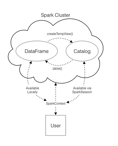
Xem cách các Spark data structure tương tác với nhau bằng nhiều cách trong biểu đồ dưới đây:

Convert thành Spark DF trực tiếp từ file .csv mà không cần thông qua pandas DF:

Now you know how to put data into Spark via pandas, but you’re probably wondering why deal with pandas at all? Wouldn’t it be easier to just read a text file straight into Spark? Of course it would!

Luckily, your SparkSession has a .read attribute which has several methods for reading different data sources into Spark DataFrames. Using these you can create a DataFrame from a .csv file just like with regular pandas DataFrames!

The variable file_path is a string with the path to the file airports.csv. This file contains information about different airports all over the world.

# Don't change this file path
file_path = "/usr/local/share/datasets/airports.csv"

# Read in the airports data
airports = spark.read.csv(file_path, header=True)

# Show the data
airport.head()

Creating columns

In this chapter, you’ll learn how to use the methods defined by Spark’s DataFrame class to perform common data operations.

Let’s look at performing column-wise operations. In Spark you can do this using the .withColumn() method, which takes two arguments. First, a string with the name of your new column, and second the new column itself.

The new column must be an object of class Column. Creating one of these is as easy as extracting a column from your DataFrame using df.colName.

Updating a Spark DataFrame is somewhat different than working in pandas because the Spark DataFrame is immutable. This means that it can’t be changed, and so columns can’t be updated in place.

Thus, all these methods return a new DataFrame. To overwrite the original DataFrame you must reassign the returned DataFrame using the method like so:

df = df.withColumn("newCol", df.oldCol + 1)

The above code creates a DataFrame with the same columns as df plus a new column, newCol, where every entry is equal to the corresponding entry from oldCol, plus one.

To overwrite an existing column, just pass the name of the column as the first argument!

# Create the DataFrame flights
flights = spark.table("flights")

# Show the head
flights.show()

# Add duration_hrs
flights = flights.withColumn("duration_hrs", flights.air_time/60)

flights.show()

Use the spark.table() method with the argument "flights" to create a DataFrame containing the values of the flights table in the .catalog. Save it as flights.
Show the head of flights using flights.show(). Check the output: the column air_time contains the duration of the flight in minutes.
Update flights to include a new column called duration_hrs, that contains the duration of each flight in hours (you'll need to divide duration_hrs by the number of minutes in an hour).

Filtering Data

Now that you have a bit of SQL know-how under your belt, it’s easier to talk about the analogous operations using Spark DataFrames.

Let’s take a look at the .filter() method. As you might suspect, this is the Spark counterpart of SQL’s WHERE clause. The .filter() method takes either an expression that would follow the WHERE clause of a SQL expression as a string, or a Spark Column of boolean (True/False) values.

For example, the following two expressions will produce the same output:

flights.filter(“air_time > 120”).show() flights.filter(flights.air_time > 120).show()

Notice that in the first case, we pass a string to .filter(). In SQL, we would write this filtering task as SELECT * FROM flights WHERE air_time > 120. Spark’s .filter() can accept any expression that could go in the WHEREclause of a SQL query (in this case, “air_time > 120”), as long as it is passed as a string. Notice that in this case, we do not reference the name of the table in the string – as we wouldn’t in the SQL request.

In the second case, we actually pass a column of boolean values to .filter(). Remember that flights.air_time > 120 returns a column of boolean values that has True in place of those records in flights.air_time that are over 120, and False otherwise.

# Filter flights by passing a string
long_flights1 = flights.filter("distance > 1000")

# Filter flights by passing a column of boolean values
long_flights2 = flights.filter(flights.distance > 1000)

# Print the data to check they're equal
long_flights1.show()
long_flights2.show()

=> Kết quả như nhau

Selecting

The Spark variant of SQL’s SELECT is the .select() method. This method takes multiple arguments - one for each column you want to select. These arguments can either be the column name as a string (one for each column) or a column object (using the df.colName syntax). When you pass a column object, you can perform operations like addition or subtraction on the column to change the data contained in it, much like inside .withColumn().

The difference between .select() and .withColumn() methods is that .select() returns only the columns you specify, while .withColumn() returns all the columns of the DataFrame in addition to the one you defined. It’s often a good idea to drop columns you don’t need at the beginning of an operation so that you’re not dragging around extra data as you’re wrangling. In this case, you would use .select() and not .withColumn().

Remember, a SparkSession called spark is already in your workspace, along with the Spark DataFrame flights.

# Select the first set of columns
selected1 = flights.select("tailnum", "origin","dest")

# Select the second set of columns
temp = flights.select(flights.origin, flights.dest, flights.carrier)

# Define first filter
filterA = flights.origin == "SEA"

# Define second filter
filterB = flights.dest == "PDX"

# Filter the data, first by filterA then by filterB
selected2 = temp.filter(filterA).filter(filterB)

Select the columns “tailnum”, “origin”, and “dest” from flights by passing the column names as strings. Save this as selected1.

Select the columns “origin”, “dest”, and “carrier” using the df.colName syntax and then filter the result using both of the filters already defined for you (filterA and filterB) to only keep flights from SEA to PDX. Save this as selected2.

Selecting II

Similar to SQL, you can also use the .select() method to perform column-wise operations. When you’re selecting a column using the df.colName notation, you can perform any column operation and the .select() method will return the transformed column. For example,

flights.select(flights.air_time/60)

returns a column of flight durations in hours instead of minutes. You can also use the .alias() method to rename a column you’re selecting. So if you wanted to .select() the column duration_hrs (which isn’t in your DataFrame) you could do

flights.select((flights.air_time/60).alias("duration_hrs"))

The equivalent Spark DataFrame method .selectExpr() takes SQL expressions as a string:

flights.selectExpr("air_time/60 as duration_hrs")

with the SQL as keyword being equivalent to the .alias() method. To select multiple columns, you can pass multiple strings.

Remember, a SparkSession called spark is already in your workspace, along with the Spark DataFrame flights.

# Define avg_speed
avg_speed = (flights.distance/(flights.air_time/60)).alias("avg_speed")

# Select the correct columns
speed1 = flights.select("origin", "dest", "tailnum", avg_speed)

# Create the same table using a SQL expression
speed2 = flights.selectExpr("origin", "dest", "tailnum", "distance/(air_time/60) as avg_speed")

Aggregating

All of the common aggregation methods, like .min(), .max(), and .count() are GroupedData methods. These are created by calling the .groupBy() DataFrame method. You’ll learn exactly what that means in a few exercises. For now, all you have to do to use these functions is call that method on your DataFrame. For example, to find the minimum value of a column, col, in a DataFrame, df, you could do

df.groupBy().min("col").show()

This creates a GroupedData object (so you can use the .min() method), then finds the minimum value in col, and returns it as a DataFrame.

Now you’re ready to do some aggregating of your own!

A SparkSession called spark is already in your workspace, along with the Spark DataFrame flights.

Ex:

flights.show()

# Find the shortest flight from PDX in terms of distance
flights.filter(flights.origin == "PDX").groupBy().min("distance").show()

# Find the longest flight from SEA in terms of air time
flights.filter(flights.origin == "SEA").groupBy().max("air_time").show()

Grouping and Aggregating I

Part of what makes aggregating so powerful is the addition of groups. PySpark has a whole class devoted to grouped data frames: pyspark.sql.GroupedData, which you saw in the last two exercises.

You’ve learned how to create a grouped DataFrame by calling the .groupBy() method on a DataFrame with no arguments.

Now you’ll see that when you pass the name of one or more columns in your DataFrame to the .groupBy() method, the aggregation methods behave like when you use a GROUP BY statement in a SQL query!

# Group by tailnum
by_plane = flights.groupBy("tailnum")

# Number of flights each plane made
by_plane.count().show()

# Group by origin
by_origin = flights.groupBy("origin")

# Average duration of flights from PDX and SEA
by_origin.avg("air_time").show()

Create a DataFrame called by_plane that is grouped by the column tailnum.
Use the .count() method with no arguments to count the number of flights each plane made.
Create a DataFrame called by_origin that is grouped by the column origin.
Find the .avg() of the air_time column to find average duration of flights from PDX and SEA.

Grouping and Aggregating II

In addition to the GroupedData methods you’ve already seen, there is also the .agg() method. This method lets you pass an aggregate column expression that uses any of the aggregate functions from the pyspark.sql.functions submodule.

This submodule contains many useful functions for computing things like standard deviations. All the aggregation functions in this submodule take the name of a column in a GroupedData table.

# Import pyspark.sql.functions as F
import pyspark.sql.functions as F

# Group by month and dest
by_month_dest = flights.groupBy("month", "dest")

# Average departure delay by month and destination
by_month_dest.avg("dep_delay").show()

# Standard deviation of departure delay
by_month_dest.agg(F.stddev("dep_delay")).show()

Import the submodule pyspark.sql.functions as F.
Create a GroupedData table called by_month_dest that's grouped by both the month and dest columns. Refer to the two columns by passing both strings as separate arguments.
Use the .avg() method on the by_month_dest DataFrame to get the average dep_delay in each month for each destination.
Find the standard deviation of dep_delay by using the .agg() method with the function F.stddev().

Joining

In PySpark, joins are performed using the DataFrame method .join(). This method takes three arguments. The first is the second DataFrame that you want to join with the first one. The second argument, on, is the name of the key column(s) as a string. The names of the key column(s) must be the same in each table. The third argument, how, specifies the kind of join to perform. In this course we’ll always use the value how=”leftouter”.

# Examine the data
print(airports.show())
print(flights.show())

# Rename the faa column
airports = airports.withColumnRenamed("faa", "dest")

# Join the DataFrames
flights_with_airports = flights.join(airports,"dest",how="leftouter")

# Examine the new DataFrame
print(flights_with_airports.show())

Examine the airports DataFrame by calling .show(). Note which key column will let you join airports to the flights table. Rename the faa column in airports to dest by re-assigning the result of airports.withColumnRenamed(“faa”, “dest”) to airports. Join the flights with the airports DataFrame on the dest column by calling the .join() method on flights. Save the result as flights_with_airports. The first argument should be the other DataFrame, airports. The argument on should be the key column. The argument how should be “leftouter”. Call .show() on flights_with_airports to examine the data again. Note the new information that has been added.